
Almost every paper starts with Table 1: Descriptive Statistics. This post describes several ways to automate the creation of these tables in Stata. I'll describe one simple method, but also two that are more flexible and allow you to create basically any type of table. I'll pay special attention to balance tables. Also, be careful when copying things over from here. If you get strange errors it might be because the quotation marks might be different than the ones you need. Basically there is the single quote ', the double quote " and this special quote `. This is usually under the tilde (~) button. This button is right underneath Escape on Windows, and to the right of the left shift button on a mac.
If you want to play along with these exact commands you can run the following code to get the same dataset this tutorial is based upon. You'll also need to create a folder called 'tables' in the same folder where you save your dofile. The full code snippet can be found here
clear
set seed 2299308
set obs 100
gen age = ceil(99*uniform())
gen male = rbinomial(1,0.8)
gen income = ceil(5000*uniform())
gen villagecode = ceil(5*uniform())
gen treated = rbinomial(1,0.5)
label var age "Age (years)"
label var male "Gender (1=male)"
label var income "Monthly Income (dollars)"
Using Esttab
Probably the best user-written package for exporting tables is Esttab. It is easy to use but also extremely flexible. Making summary statistics is pretty simple using esttab. You can install it by typing this in Stata:
ssc install esttabEsttab always works in two steps: first you "post" the results you care about to memory, and then you use esttab to output a formatted table. The simplest use looks like this:
eststo clear
estpost summarize age male income
esttab using "tables/table1.rtf", replace ///
cells("count(fmt(a2)) mean sd min max") label ///
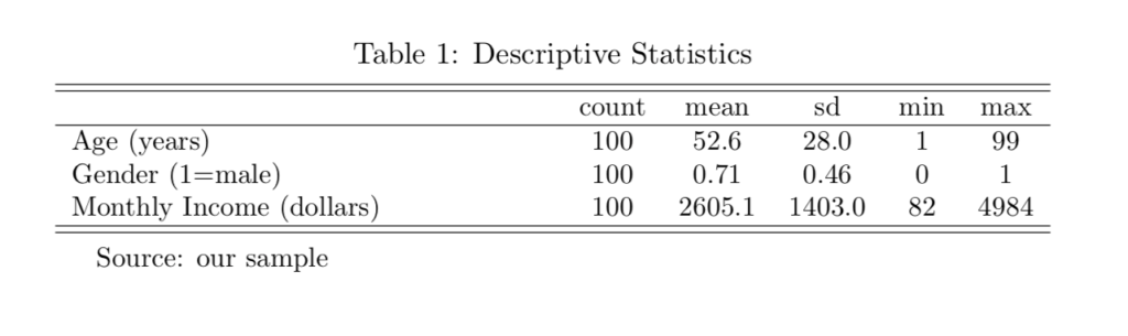
title("Table 1: Descriptive Statistics") nomtitle nonumber noobs We first clear all results from the memory. Then we post the results for a list of variables. Then we call esttab. We include a location where the table should be put. The file extension is .rtf which I like because Word opens it natively but you can also view it using Preview on a mac. By specifying cells we can determine for which statistics data should be posted. In this case count (number of observations), mean, standard deviation, minimum and maximum. We drom model titles (nomtitle), model numbers (nonumber) and observations (noobs).
The optimal way is to export directly to a .tex document, which can be automatically added in your paper in Latex. The code is similar:
eststo clear
estpost summarize age male income
esttab using "tables/table1.tex", replace label substitute(# \#) ///
    fragment nomtitle nonumber noobs cells("count(fmt(a2)) mean sd min max")
Only the esttab command is different: we remove the title (we'll add that in Latex). We substitute # with \#. We also add the fragment command which gets you an extremely minimal .tex file: this allows us to define the table environment etc in Latex. Then in Latex we use the following code:
\documentclass[11pt, a4paper]{article}
\usepackage{tabularx}
\usepackage{threeparttable}

\def\sym#1{\ifmmode^{#1}\else\(^{#1}\)\fi}

\begin{document}

\begin{table}[!htbp]\centering
    \begin{threeparttable}
        \small
        \caption{Descriptive Statistics}
        \label{tab:descriptives}
        \begin{tabularx}{\textwidth}{X *{5}{c}}
            \hline\hline
            \input{tables/table1.tex}
            \hline\hline
        \end{tabularx}
        \begin{tablenotes}
            \item Source: our sample
        \end{tablenotes}
    \end{threeparttable}
\end{table}

\end{document}
I like to use the package tabularx because it allows line wrapping if you have very long variable labels. I use threeparttable as the environment because it allows you to add notes and captions and it'll all be nicely aligned. The \def command is required for Stata tables: it's related to some symbols Stata outputs in the table.
We then wrap the table in a table and threeparttable environment, add a label and a caption. The main work is under tabularx. We set the width to the text width. The first column is an "X" column: this means the line can wrap if you have long labels. The rest are simply centered. We add horizontal lines before and after the table, and add the table using \input. We also add some notes. This is what it'll look like:
You can expand the list of statistics you want to output:
cells("count(fmt(a2) label(N)) mean(label(Mean)) sd(label(SD)) p50(label(Median)) min(label(Min)) max(label(Max))")This is somewhat more complicated: now we also add the median (p50), and also add labels so it will display nicely. See the helpfile for estpost to see the full list of statistics you can add. Note that if you want to add the median you will need to add the option "detail" to the eestpost summarize command:
estpost summarize age male income, detailUsing Outreg
While Esttab is great, it's not very flexible. For example, you can't create a balance table that has clustered standard errors for the test of differences. And if you want any additional statistics that's impossible. Outreg is able to do this. The syntax is generally a bit more complicated than esttab, but you get tables that look really great in Latex (and Word is also possible of course). Outreg was not developed for a while, which prompted the creation of outreg2 (which I've seen people use a lot). Development of outreg was picked up again recently and it's really great now. Much better than outreg2 which hasn't been updated in a while. Install it like this:
ssc install outregThe following describes how you can create a balance table for a treatment and control group, and the test the difference with clustered standard errors. We do this by first creating a table with differences and then we merge this with the descriptive statistics. First we make the differences column:
global DESCVARS age male income
mata: mata clear

* First test of differences
local i = 1

foreach var in $DESCVARS {
    reg `var' treated, vce(cluster villagecode)
    outreg, keep(treated)  rtitle("`: var label `var''") stats(b) ///
        noautosumm store(row`i')  starlevels(10 5 1) starloc(1)
    outreg, replay(diff) append(row`i') ctitles("",Difference ) ///
        store(diff) note("")
    local ++i
}
outreg, replay(diff)
We use the list of descriptive variables often, so I put them in a global to easily reference them. We clear mata beforehand because we'll be using it later. We first create a table of differences. We use a counter (i) to track the variable we are at. We loop over our list of variables and then run the the test we want to (a regression with clustered SEs). We then call outreg and we say we want to keep only the treatment variable. As rowtitles (rtitle) we add the variable label. We keep only statistics for the coefficient (b). noautosumm removes the r-squared etc. We store it as row`i' (so row1 for the first variable). Finally we change the significance level to standard levels and we write the star next to the coefficient.
Then we call outreg again: this is where we combine the rows to make the difference column. replay means the table named diff is called again (on the first time around this is undefined, fortunately outreg just carries on). We append the row we just created. We add column titles (first empty, then Difference). We store it under the name diff and do not add any notes. Finally we increment the counter once and move on to the next variable. At the end we call the full table.
So at the end of this loop outreg will have created a table that consists of one column of variable labels, one column examining difference between the treatment groups. The number of rows is equal to the number of variables you put in $DESCVARS.
Next, we move on to the summary statistics. We put the statistics we are interested in in a matrix, and then call this using frmttable, which is a part of outreg. This is very flexible. We could also add the intra-cluster correlation in this loop. This is what it looks like:
* Then Summary statistics
local count: word count $DESCVARS
mat sumstat = J(`count',6,.)

local i = 1
foreach var in $DESCVARS {
    quietly: summarize `var' if treated==0
    mat sumstat[`i',1] = r(N)
    mat sumstat[`i',2] = r(mean)
    mat sumstat[`i',3] = r(sd)
    quietly: summarize `var' if treated==1
    mat sumstat[`i',4] = r(N)
    mat sumstat[`i',5] = r(mean)
    mat sumstat[`i',6] = r(sd)
    local i = `i' + 1
}
frmttable, statmat(sumstat) store(sumstat) sfmt(g,f,f,g,f,f)
First we count the number of words in $DESCVARS: this tells us how large the matrix should be (equal to the number of variables in $DESCVARS). We define a matrix called sumstat with 6 columns and however many variables are in $DESCVARS (3 in this example). We start a new counter i. We again loop over the variables. We first summarize the results for the control group (if treated==0). Summarize stores several numbers in the memory which we can access. We store these in the matrix we just created. The first number in square brackets is the row number (i here), and the second the column. We do the same for the treatment group. Finally we call frmttable to convert the matrix to a table outreg can use. Statmat converts the matrix sumstat to a table. We store this under the name sumstat. Finally we format the numbers. g for number of observations and f for all other numbers. This is because number of observations will always be an integer.
Now we have two tables that outreg can access: sumstat and diff. Finally we put these together using outreg and export it to a .tex file:
outreg using "tables/balance", ///
    replay(sumstat) merge(diff) tex nocenter note("") fragment plain replace ///
    ctitles("", Control, "", "", Treatment, "", "", "" \ "", n, mean, sd, n, mean, sd, Diff) ///
    multicol(1,2,3;1,5,3)
We first say where we want to save the file. We replay sumstat: this will cause it to be on the left. We merge in the table diff. This will simply jam the tables together. Be very careful that the global $DESCVARS is not changed in between making the two tables: otherwise the two won't match up. We export to a tex file. Then we remove some fluff to get the table as minimal as possible: nocenter, note("") fragment, plain. Next we add column titles. The top row is control and treatment only: we put those in the second and fifth column. Then comes the second row: here we put n, mean etc. Finally we make multicolumns: this means that control is attached to the first n, mean and sd. We do this for the first row, starting from the second column, and do it for 3 columns (1,2,3). The same holds for treatment, but that one starts in column 5 (1,5,3). Here I'm exporting to .tex. If you want a word (.doc) document you need to remove the 'tex' and 'fragment' options.
Finally we enter it in a latex document:
\documentclass{article}
\usepackage[T1]{fontenc}

\begin{document}

\begin{table}[!htbp]\centering
    \scriptsize
    \caption{Descriptive Statistics and Balance}
    \label{tab:balance}
    \input{tables/balance.tex}
    \begin{flushleft}
        \noindent Table shows averages for baseline. The Diff column is the coefficient of a simple regression of treatment status on the variable, with clustered standard errors at the village level. Stars indicate whether this difference is significant.

        \noindent * p < 0.10, ** p < 0.05, *** p < 0.01.
    \end{flushleft}
\end{table}

\end{document}
The actual code is simpler: we only need to use a package to get < and > to work. Unfortunately outreg likes to add it's own table environment, and this can't be removed automatically. Therefore we cannot use Threeparttable, so the notes will not be aligned as well. I've e-mailed the author of outreg if this can be fixed, but he hasn't found the time to fix it yet. We add a flushleft environment to add notes to the table. And this is how it ends up looking:
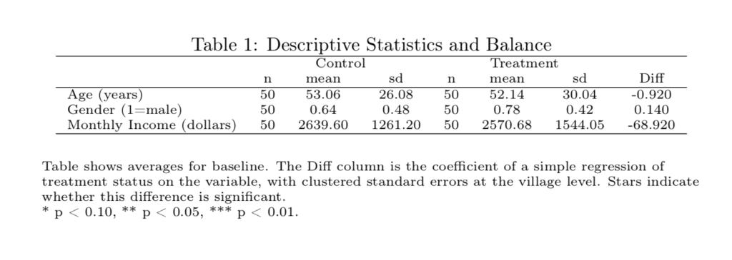
Pretty good, except for the notes.
Using Postfiles
There is another way I used in the past: using postfiles. I think the outreg method actually supersedes it as it is as flexible, but allows nicer formatting and exporting to .tex. It might be problematic if you are not running any regressions as this is where the variable names come from in the outreg method.
How postfiles work is that you loop over all your variables and write the statistics you care about to a background file (the postfile). This is fully flexible. Any kind of statistic you can calculate in Stata you could add to this method. Here we'll make a table of N, mean, sd and intra-cluster correlation (great if someone want to use your data for power calculations for a clustered randomized study). What it looks like in Stata:
tempname memhold
tempfile stats_icc
postfile `memhold' str60 Variable N Mean SD ICC   using "`stats_icc'"

foreach var in age male income {
    scalar varlabel = `"`: var label `var''"'
    quietly: su `var'
    scalar N =`r(N)'
    scalar Mean = `r(mean)'
    scalar SD = `r(sd)'
    quietly: loneway `var' villagecode
    scalar ICC = `r(rho)'
    post `memhold' (varlabel) (N) (Mean) (SD) (ICC)
    scalar drop _all
}

postclose `memhold'
use "`stats_icc'", clear

*Export to csv.
export delimited using "tables/descriptives_icc.csv", replace
We first define a temporary name and a temporary file. Then we define what the postfile will look like. It is linked to memhold. Then we write the column titles: The first column is called Variable and is a string with length 60. Next are N, Mean, SD and ICC (numbers are the default so we don't need to specify). We write this in a temporary file called stats_icc. The weird quotation marks are required because it is a temporary file. Note that you have to run this entire piece of code in one go because the temporary file is separate for each "run".
Then we loop over all variables again. Now we define a set of scalars. Scalars simply hold one value (can be text or numbers). We add the variable label to the scalar varlabel. Then we summarize the variable and add the mean, sd and N to further scalars. The we use the loneway command to calculate the ICC, and again put this in a scalar. Then we "post" these results. Each thing you want to post has to be enclosed in brackets, and it has to match the order we defined earlier. At the end of the loop we drop all scalars and move on to the next variable.
Then we close the postfile. You have to do this. After closing it will save the dataset you just created to the temporary file you defined. We then open this. This is just a Stata dataset with five variables: Variable, N, Mean, SD and ICC. You can just export this to a .csv or excel file and then copy it to Word or include/input it in a Latex file. While the flexibility is great, this method has some issues. You can't easily add stars if you calculate some kind of p-value. You also don't have control over the number of digits after the decimal point, so you'll need to fix that manually.
Other methods
I've seen a Stata package called BALANCETABLE (on SSC) that promises to make balance tables easily and exports to .rtf and .tex. It's Stata 14 and up only though so I haven't been able to use it.